Datoteka:Airflow-Obstructed-Duct.png
Vidi sliku u punoj veličini (1.270 × 907 piksela, veličina datoteke: 85 KB, MIME tip: image/png)
| Ova je datoteka sa Zajedničkog poslužitelja i mogu je rabiti drugi projekti. Opis s njezine stranice s opisom datoteke prikazan je ispod. |
Sažetak

|
Dostupna je vektorska inačica (SVG) ove slike. Trebala bi se koristiti umjesto ove rasterske slike ako je kvalitetnija.
File:Airflow-Obstructed-Duct.png → File:N S Laminar.svg
Za više informacija o vektorskoj grafici, pročitajte o prelasku Zajedničkog poslužitelja na SVG. Također pročitajte informacije o podršci MediaWiki softvera slikama u SVG formatu. |
 |
| Opis |
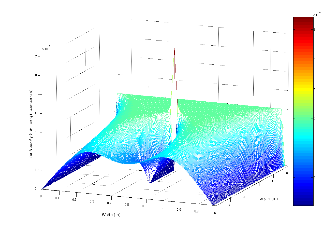
A simulation using the navier-stokes differential equations of the aiflow into a duct at 0.003 m/s (laminar flow). The duct has a small obstruction in the centre that is parallel with the duct walls. The observed spike is mainly due to numerical limitations. This script, which i originally wrote for scilab, but ported to matlab (porting is really really easy, mainly convert comments % -> // and change the fprintf and input statements) Matlab was used to generate the image.
%Matlab script to solve a laminar flow
%in a duct problem

%Constants
inVel = 0.003; % Inlet Velocity (m/s)
fluidVisc = 1e-5; % Fluid's Viscoisity (Pa.s)
fluidDen = 1.3; %Fluid's Density (kg/m^3)

MAX_RESID = 1e-5; %uhh. residual units, yeah...
deltaTime = 1.5; %seconds?
%Kinematic Viscosity
fluidKinVisc = fluidVisc/fluidDen;

%Problem dimensions
ductLen=5; %m
ductWidth=1; %m

%grid resolution
gridPerLen = 50; % m^(-1)
gridDelta = 1/gridPerLen;
XVec = 0:gridDelta:ductLen-gridDelta;
YVec = 0:gridDelta:ductWidth-gridDelta;

%Solution grid counts
gridXSize = ductLen*gridPerLen;
gridYSize = ductWidth*gridPerLen;

%Lay grid out with Y increasing down rows
%x decreasing down cols
%so subscripting becomes (y,x) (sorry)
velX= zeros(gridYSize,gridXSize);
velY= zeros(gridYSize,gridXSize);
newVelX= zeros(gridYSize,gridXSize);
newVelY= zeros(gridYSize,gridXSize);

%Set initial condition

for i =2:gridXSize-1
for j =2:gridYSize-1
velY(j,i)=0;
velX(j,i)=inVel;
end
end

%Set boundary condition on inlet
for i=2:gridYSize-1
velX(i,1)=inVel;
end

disp(velY(2:gridYSize-1,1));

%Arbitrarily set residual to prevent
%early loop termination
resid=1+MAX_RESID;

simTime=0;

while(deltaTime)
 count=0;
while(resid > MAX_RESID && count < 1e2)
 count = count +1;
for i=2:gridXSize-1
for j=2:gridYSize-1
newVelX(j,i) = velX(j,i) + deltaTime*( fluidKinVisc / (gridDelta.^2) * ...
(velX(j,i+1) + velX(j+1,i) - 4*velX(j,i) + velX(j-1,i) + ...
velX(j,i-1)) - 1/(2*gridDelta) *( velX(j,i) *(velX(j,i+1) - ...
velX(j,i-1)) + velY(j,i)*( velX(j+1,i) - velX(j,i+1))));

newVelY(j,i) = velY(j,i) + deltaTime*( fluidKinVisc / (gridDelta.^2) * ...
(velY(j,i+1) + velY(j+1,i) - 4*velY(j,i) + velY(j-1,i) + ...
velY(j,i-1)) - 1/(2*gridDelta) *( velY(j,i) *(velY(j,i+1) - ...
velY(j,i-1)) + velY(j,i)*( velY(j+1,i) - velY(j,i+1))));
end
end

%Copy the data into the front
for i=2:gridXSize - 1
for j = 2:gridYSize-1
velX(j,i) = newVelX(j,i);
velY(j,i) = newVelY(j,i);
end
end

%Set free boundary condition on inlet (dv_x/dx) = dv_y/dx = 0
for i=1:gridYSize
velX(i,gridXSize)=velX(i,gridXSize-1);
velY(i,gridXSize)=velY(i,gridXSize-1);

    end

    %y velocity generating vent
    for i=floor(2/6*gridXSize):floor(4/6*gridXSize)
        velX(floor(gridYSize/2),i) = 0;
        velY(floor(gridYSize/2),i-1) = 0;
    end

%calculate residual for
%conservation of mass
resid=0;
for i=2:gridXSize-1
for j=2:gridYSize-1
%mass continuity equation using central difference
%approx to differential
resid = resid + (velX(j,i+ 1)+velY(j+1,i) - ...
(velX(j,i-1) + velX(j-1,i)))^2;
end
end

resid = resid/(4*(gridDelta.^2))*1/(gridXSize*gridYSize);
fprintf('Time %5.3f \t log10Resid : %5.3f\n',simTime,log10(resid));


simTime = simTime + deltaTime;
end
mesh(XVec,YVec,velX)
deltaTime = input('\nnew delta time:');
end
%Plot the results
mesh(XVec,YVec,velX)
|
| Datum | 24. veljače 2007. (izvorni datum postavljanja) |
| Izvor | Prebačeno s en.wikipedia na Zajednički poslužitelj . |
| Autor | User A1 na Wikipediji na engleskom jeziku |
Licencija
| Ovo djelo je u javno vlasništvo izdao autor: User A1 na Wikipediji na engleskom jeziku. To vrijedi za cijeli svijet. U nekim državama to nije pravno moguće; ako je tako: User A1 daje svima prava da koriste ovo djelo za bilo koju svrhu, bez ikakvih uvjeta, osim ako takvi uvjeti nisu propisani zakonom. |
Izvorna evidencija postavljanja
- 2007-02-24 05:45 User A1 1270×907×8 (86796 bytes) A simulation using the navier-stokes differential equations of the aiflow into a duct at 0.003 m/s (laminar flow). The duct has a small obstruction in the centre that is paralell with the duct walls. The observed spike is mainly due to numerical limitatio
Povijest datoteke
Kliknite na datum/vrijeme kako biste vidjeli datoteku kakva je tada bila.
| Datum/Vrijeme | Minijatura | Dimenzije | Suradnik | Komentar | |
|---|---|---|---|---|---|
| sadašnja | 17:52, 1. svibnja 2007. | | 1.270 × 907 (85 KB) | Smeira | {{Information |Description=A simulation using the navier-stokes differential equations of the aiflow into a duct at 0.003 m/s (laminar flow). The duct has a small obstruction in the centre that is paralell with the duct walls. The observed spike is mainly |
Uporaba datoteke
Na ovu sliku vode poveznice sa sljedećih stranica:
Globalna uporaba datoteke
Sljedeći wikiji rabe ovu datoteku:
- Uporaba na anp.wikipedia.org
- Uporaba na ar.wikipedia.org
- Uporaba na ba.wikipedia.org
- Uporaba na bg.wikipedia.org
- Uporaba na bn.wikipedia.org
- Uporaba na ca.wikipedia.org
- Uporaba na ckb.wikipedia.org
- Uporaba na cs.wikipedia.org
- Uporaba na de.wikipedia.org
- Uporaba na en.wikipedia.org
- Uporaba na en.wikiquote.org
- Uporaba na es.wikipedia.org
- Uporaba na fa.wikipedia.org
- Uporaba na he.wikipedia.org
- Uporaba na hif.wikipedia.org
- Uporaba na hi.wikipedia.org
- Uporaba na hy.wikipedia.org
- Uporaba na id.wikipedia.org
- Uporaba na jv.wikipedia.org
- Uporaba na ko.wikipedia.org
- Uporaba na ko.wikiversity.org
- Uporaba na map-bms.wikipedia.org
- Uporaba na ms.wikipedia.org
- Uporaba na mwl.wikipedia.org
- Uporaba na pt.wikipedia.org
- Isaac Newton
- Equação diferencial
- Equações de Navier-Stokes
- Equação diferencial linear
- Equação diferencial de Bernoulli
- Equação diferencial de d'Alembert
- Decaimento exponencial
- Equação de Laplace
- Equação diferencial parcial
- Equação de Poisson
- Equação do calor
- Lema de Grönwall
- Teorema de Picard-Lindelöf
- Método de Runge-Kutta
- Equação de Mason-Weaver
- Equação do pêndulo
- Equação de onda
- Método Multigrid
Pogledajte globalnu uporabu ove datoteke.